Excel dynamic arrays explained: Practical examples in ONLYOFFICE

If you’ve ever spent time manually copying formulas down hundreds of rows or wrestling with complex Ctrl+Shift+Enter array entries, Excel dynamic arrays are about to change your workflow. A single dynamic array formula automatically expands to fill as many cells as the result requires — no repetition, no manual updates. This guide covers everything you need to know about them.

What are dynamic arrays in Excel?

A dynamic array is a range of values produced by a single formula that automatically “spills” its results into multiple adjacent cells.

Before dynamic arrays, multi-cell results required either copying formulas manually or using legacy CSE array formulas (entered with Ctrl+Shift+Enter), which were locked to a fixed output size and couldn’t grow or shrink with your data.

Dynamic array formulas remove that constraint entirely. Just type the formula, press Enter, and Excel fills in the rest. If your source data grows, the spill range expands automatically. If data is removed, it contracts.

Example: =SORT(UNIQUE(A2:A100)) produces a sorted, deduplicated list in a single cell — no CSE, no helper columns.

How dynamic arrays work: Spill behavior and core functions

Spill behavior

When a dynamic array formula produces multiple results, Excel places them in a contiguous block called the spill range. A few things to know:

• Only the top-left cell contains the formula; the rest display spilled values.
• The spill range updates automatically as source data changes.
• If any cell in the output area is occupied, Excel returns a #SPILL! error — clear the blockage to fix it.
• Use the # operator to reference a whole spill range: =SUM(A2#) sums everything spilled by the formula in A2, and adjusts automatically if that range grows.
• Dynamic array formulas do not work inside tables — place them in the regular grid.

Core dynamic array functions

Let’s have a look at the most important functions using ONLYOFFICE Spreadsheet Editor

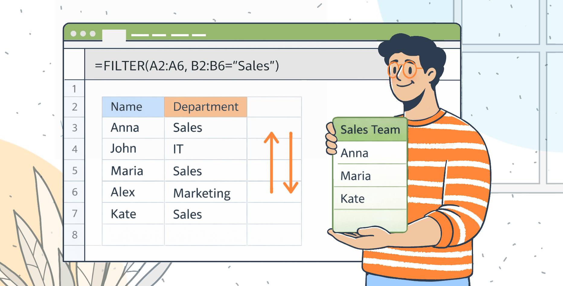
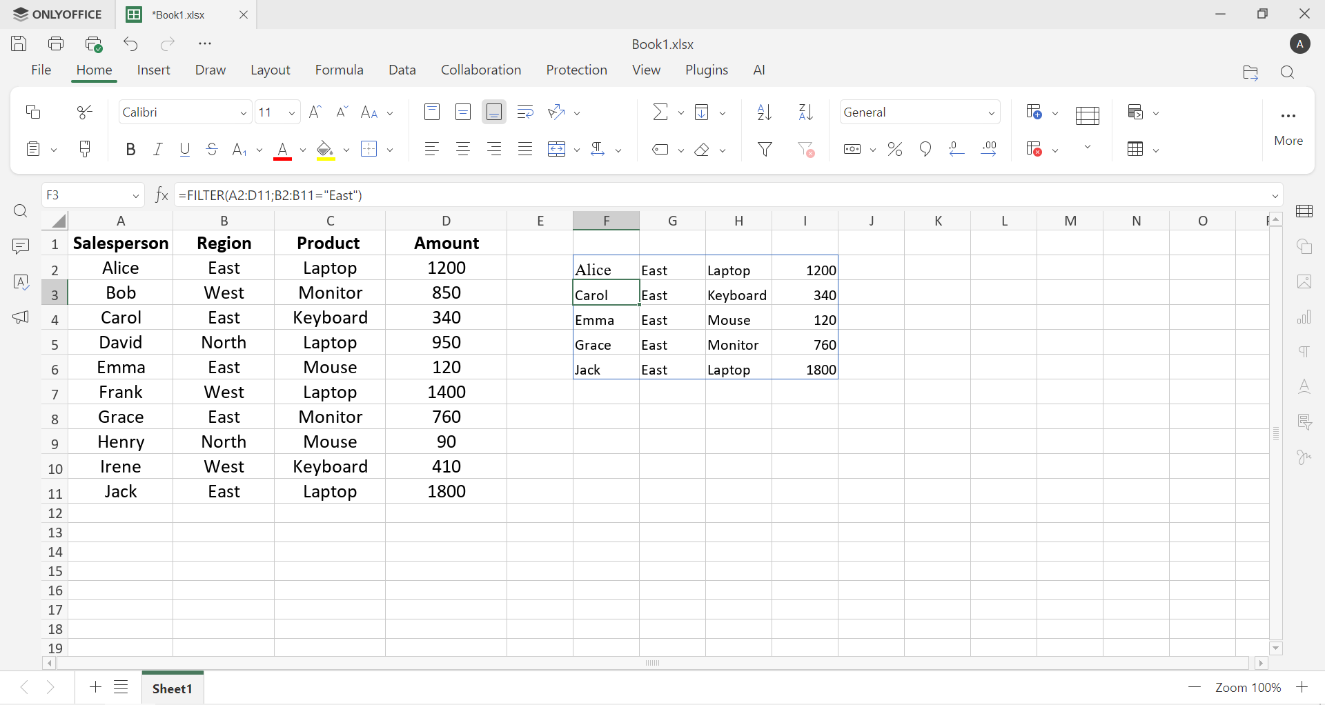
1. FILTER — extracts rows that match a condition:

=FILTER(A2:D200, B2:B200="East")

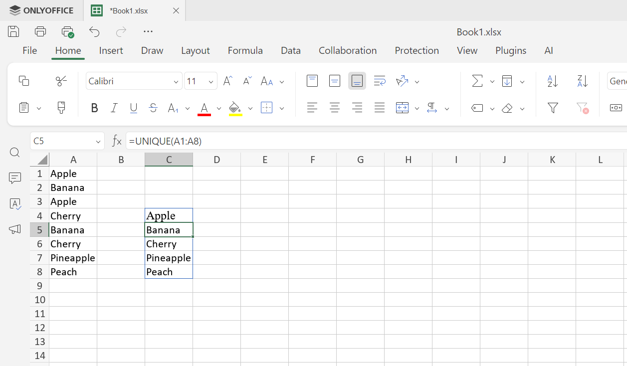
2. UNIQUE — returns a deduplicated list:

=UNIQUE(A1:A8)

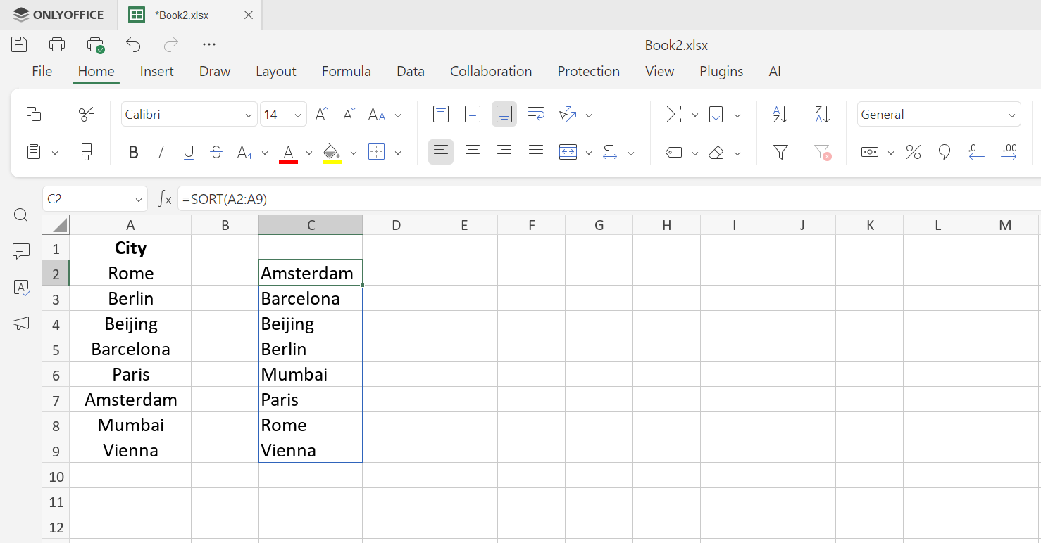
3. SORT — sorts a range with a formula:

=SORT(A2:A9)

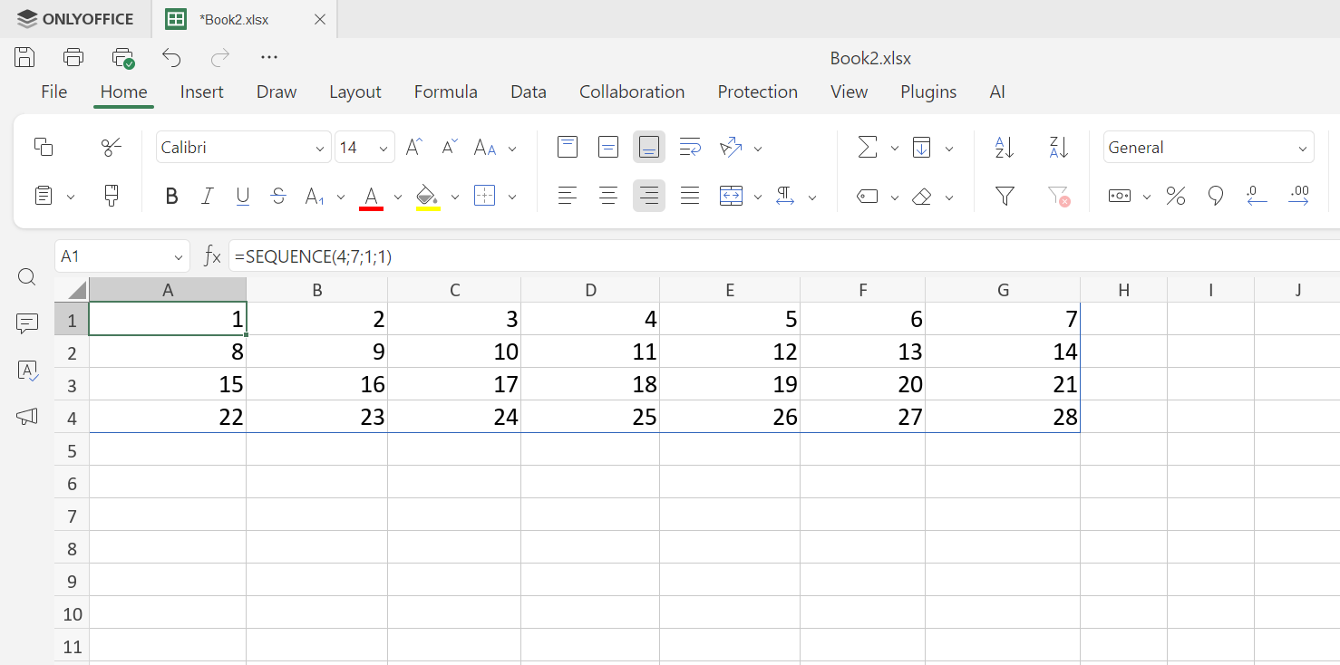
4. SEQUENCE — generates a grid of sequential numbers:

=SEQUENCE(4; 7; 1; 1)

5. RANDARRAY — fills a range with random numbers:

=RANDARRAY(5; 3; 1; 100; 1)

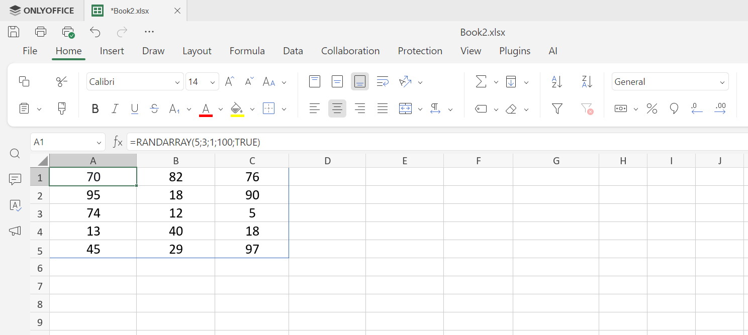
Set the last argument to 1 for integers. Recalculates on every sheet refresh.

6. XLOOKUP — the modern alternative to VLOOKUP, capable of returning multiple columns at once:

=XLOOKUP(G2, A2:A200, B2:D200, "Not found")

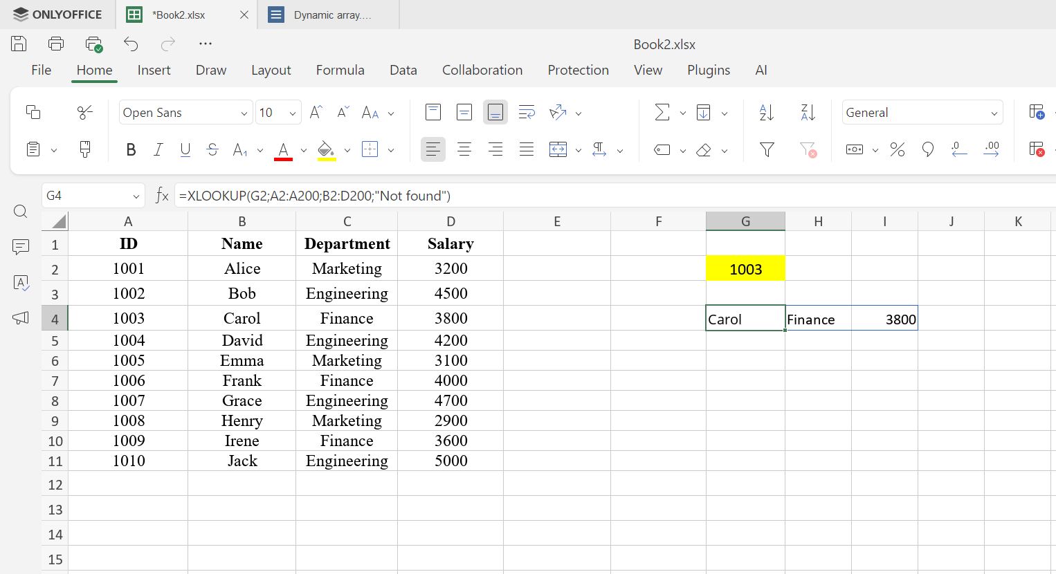
The result spills across columns automatically. For more on lookup formulas, see our Excel LOOKUP function guide. Understanding how function arguments work is especially helpful when nesting these functions together.

Benefits and considerations of dynamic arrays

Why they’re worth it

• Automatic expansion — output adjusts to data size with no manual intervention.
• Fewer formulas — one formula replaces dozens of copies, reducing file complexity.
• Better readability — easier to audit a single source formula than hunt through 500 identical copies.
• Fewer errors — no more broken references or subtly different formulas from manual copying.
• Composability — functions chain naturally: =SORT(UNIQUE(FILTER(A2:A100, B2:B100="Q1"))).

Practical Considerations

• Layout planning — leave enough empty space below and to the right of your formula for the spill range.
• Compatibility — these functions require Excel 365, Excel 2021, or ONLYOFFICE Docs. Older Excel versions don’t support them.
• Large ranges — applying UNIQUE or FILTER to entire columns can slow recalculation; limit the input range to actual data rows.

Example of dynamic arrays and combinations

Once you’re comfortable with individual functions, the real power of dynamic arrays comes from chaining them together. This is a scenarios that goes beyond the basics.

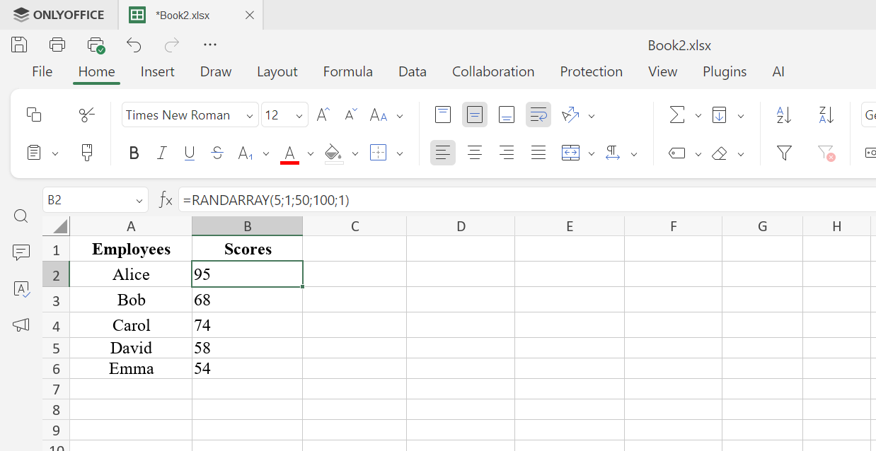
Performance scorecard with RANDARRAY and RANK

Scenario: you want to simulate performance scores for a team and automatically assign each person a ranking position.

Set up employee names in A2:A6.

In B2, generate random scores between 50 and 100:

=RANDARRAY(5; 1; 50; 100; 1)

Once you’re happy with the scores, paste them as values (Ctrl+Shift+V → Values only) to prevent them from recalculating as you work.

In C2, assign each score a rank position:

=RANK(B2; $B$2:$B$6; 0)

Drag down to C6. The $ locks the reference range so every score is compared against all five — without it, each row would rank against itself only.

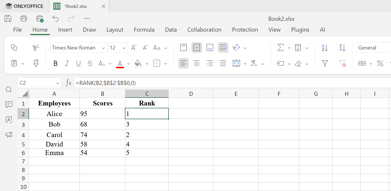
The result is a three-column scorecard showing each employee, their score, and their position in the team ranking — updated automatically whenever scores change. No manual sorting, no helper columns.

Use cases: Who benefits most?

Data analysts use FILTER, UNIQUE, and SORT to build self-updating summaries without helper columns or pivot tables.

Finance teams build reports that refresh automatically as new transactions are added, and use SEQUENCE for fiscal period structures.

Project managers create task trackers that dynamically list active projects, unique assignees, or overdue items — no macros required.

When to reach for dynamic arrays:

• Reports and dashboards that need live data without manual updates
• Unique value lists for dropdowns or summaries
• Ranked or filtered views that shouldn’t disturb source data
• Multi-column lookups with XLOOKUP

Get ONLYOFFICE and start using dynamic arrays today

Dynamic arrays are one of the most practical upgrades in modern spreadsheet work. One formula replaces dozens, results update on their own, and your files stay clean and auditable.

Start small: swap a VLOOKUP column for XLOOKUP, use UNIQUE for your next dropdown, or build one FILTER summary instead of a static copy-paste table. The shift in how you think about spreadsheets happens quickly.

Try the full dynamic array experience in creating a free ONLYOFFICE DocSpace account or offline by downloading the free desktop application for your PC or laptop with Windows, Linux or macOS:

START ONLINE   GET DESKTOP APP