Popular spreadsheet formulas: A guide

Spreadsheets are part of everyday work: expenses planning, performance analysis or detailed forecasts. What makes them truly useful isn’t the grid itself, but the logic that connects the data inside it.

In this article, we’ll look at some of the most widely used spreadsheet formulas and see how they can be applied in real scenarios.

To understand why formulas matter so much, it’s important to look at what they actually enable you to do. They transform a simple table into a functional system where numbers react, update, and interact automatically. With the right functions, you can calculate time intervals, count specific entries, retrieve matching values from large datasets, and generate results that adjust instantly when the underlying data changes.

In the following sections, each function will be illustrated step by step using ONLYOFFICE Spreadsheet Editor.

1. SUM – Adding numbers

The SUM function is fundamental for any spreadsheet work. It allows you to quickly add numbers from single cells, ranges, or even multiple ranges.

Syntax:

=SUM(number1, number2, ...)

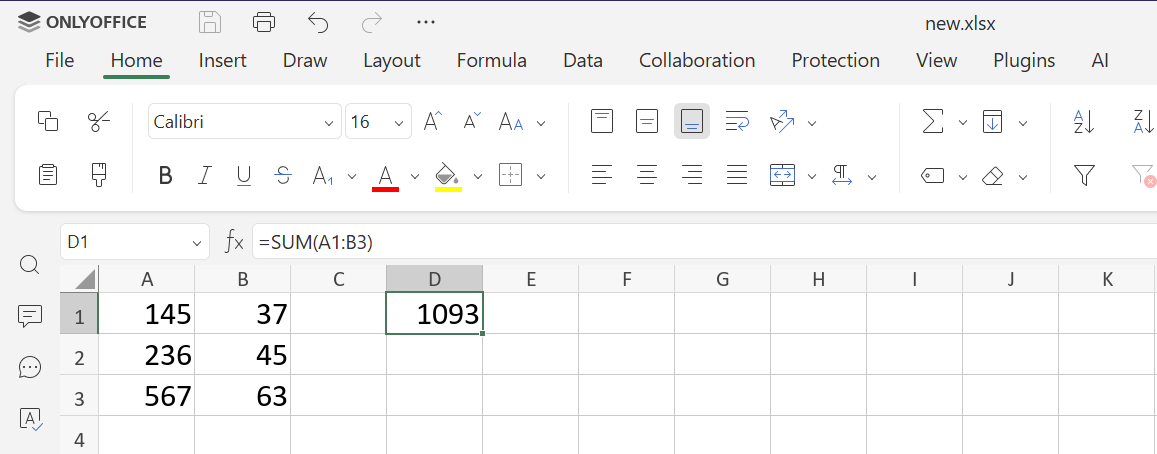
Practical use: Use SUM to calculate monthly expenses, weekly sales totals, or aggregate any numeric dataset.

Advanced tip: Combine SUM with conditional logic:

=SUM(IF(B2:B10>50, B2:B10, 0))

This formula sums only numbers greater than 50. In ONLYOFFICE, array formulas require pressing Ctrl+Shift+Enter.

2. AVERAGE – Finding the mean

AVERAGE calculates the arithmetic mean of selected numbers, ignoring blank cells but including zeros.

Syntax:

=AVERAGE(number1, number2, ...)

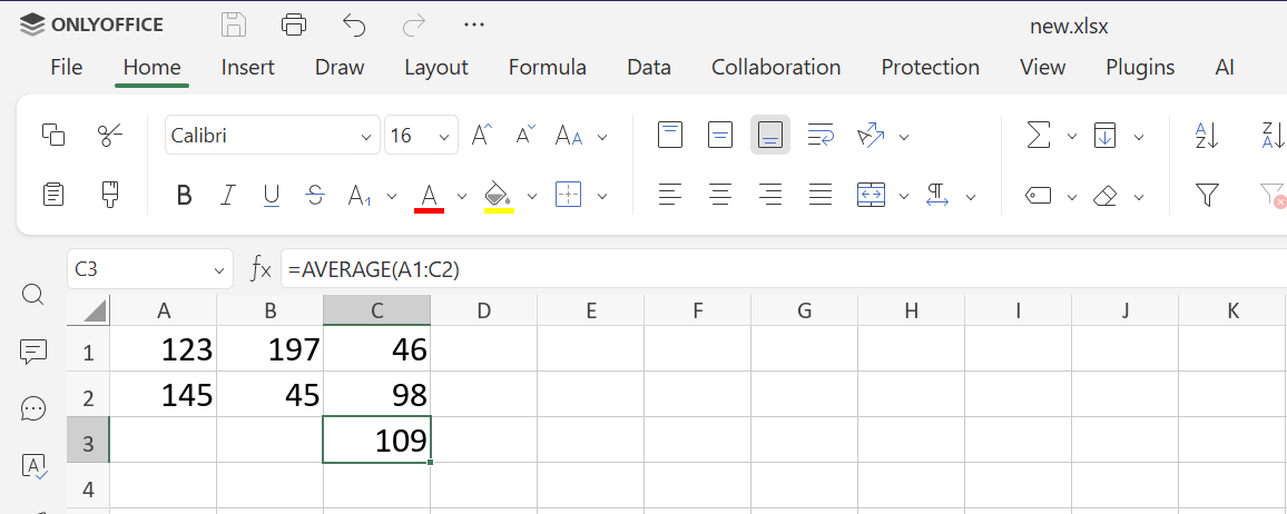
Practical use: Measuring average employee performance, average revenue per month, or average temperature readings.

Advanced tip: AVERAGEIF calculates averages based on a condition:

=AVERAGEIF(C1:C10, ">100")

This computes the average only for cells with values greater than 100.

3. IF – Conditional logic

The IF function introduces logic into spreadsheets. It returns one value if a condition is true, another if false.

Syntax:

=IF(condition, value_if_true, value_if_false)

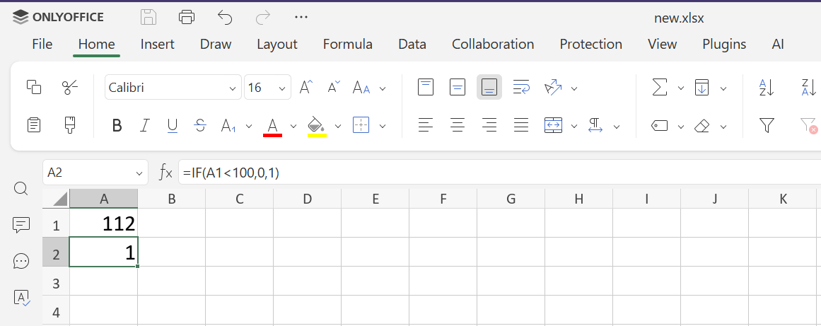
Practical use: Classifying data, evaluating conditions like budget limits, or generating dynamic messages in reports.

Advanced tip: Combine IF with other formulas:

=IF(SUM(A1:A5)>100, "Over Budget", "Within Budget")

4. VLOOKUP – Vertical Lookup

VLOOKUP searches for a value in the first column of a table and returns a corresponding value from another column.

Syntax:

=VLOOKUP(search_key, range, index, [is_sorted])

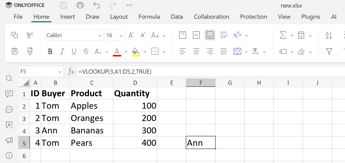
Practical use: Quickly retrieve product prices, employee details, or customer information from large tables without manually scanning rows.

Advanced tip: Always use FALSE for exact matches to prevent incorrect matches when the first column isn’t sorted. For more flexibility, use INDEX & MATCH which allow lookup in any column, not just the first.

Learn all the details about the formula in our dedicated post.

5. CONCAT / CONCATENATE – Joining text

CONCAT joins text from multiple cells or values into one string.

Syntax:

=CONCAT(text1, text2, ...)

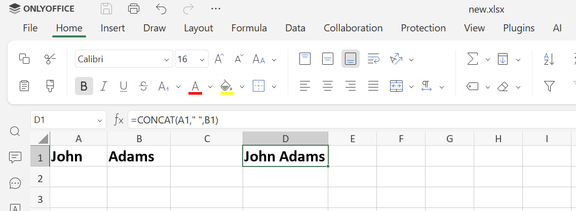
Practical use: Creating full names, addresses, formatted codes, or custom labels.

Advanced tip: Combine with TEXT for formatting numbers in concatenation:

=CONCAT("Total: $", TEXT(E2, "0.00"))

6. LEN – Counting characters

LEN counts all characters in a cell, including spaces.

Syntax:

=LEN(text)

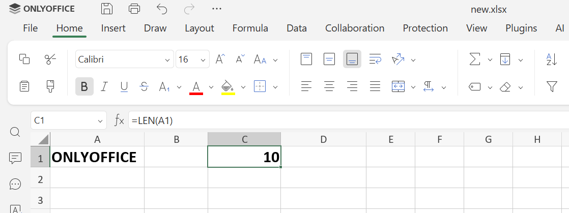
Practical use: Ensuring text does not exceed limits, validating codes, or analyzing input lengths.

Advanced tip: Combine with TRIM to remove extra spaces:
=LEN(TRIM(F2))

7. TODAY and NOW – Dynamic dates and times

TODAY returns the current date; NOW returns current date and time. Both update automatically when the spreadsheet recalculates.

Syntax:

=TODAY()

=NOW()

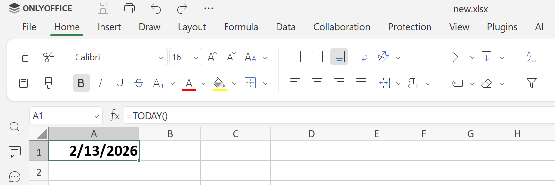
Practical use: Tracking deadlines, scheduling, generating dynamic reports.

Advanced tip: Combine with other functions like IF or NETWORKDAYS to create dynamic schedules, countdowns, or alerts that update automatically each day.

8. NETWORKDAYS – Counting workdays

NETWORKDAYS counts working days between two dates, excluding weekends and optional holidays.

Syntax:

=NETWORKDAYS(start_date, end_date, [holidays])

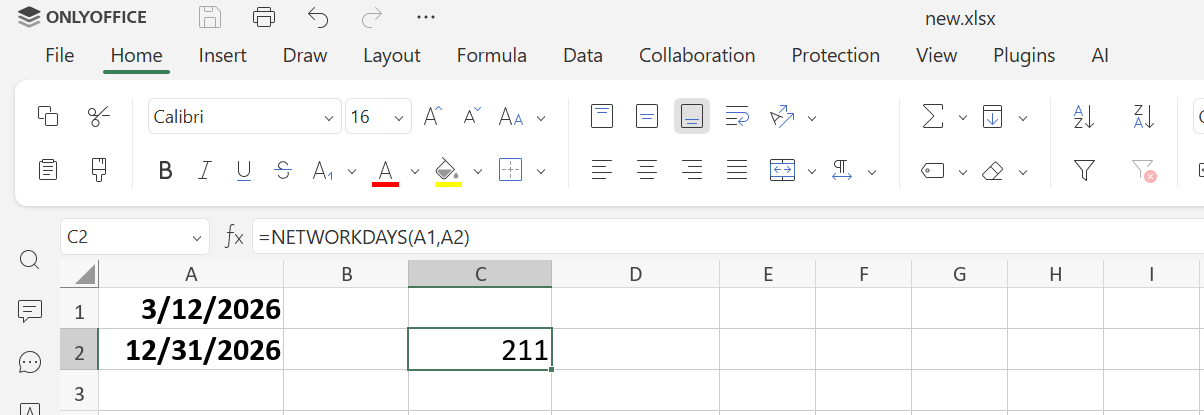
Practical use: Project timelines, HR calculations, task scheduling.

Advanced tip: Include a custom list of holidays to get precise working day counts for multiple regions or project-specific calendars.

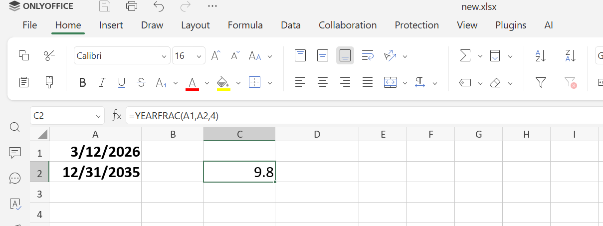
9. YEARFRAC – Fraction of a year

YEARFRAC calculates how much of a full year passes between two dates and returns the result as a decimal number (for example, 0.5 for half a year).

Syntax:

=YEARFRAC(start_date, end_date, [basis])

Practical use: Interest calculation, tenure tracking, depreciation schedules.

Advanced tip: Use the optional basis argument to adjust calculations for different day count conventions in finance, such as 30/360 or actual/360.

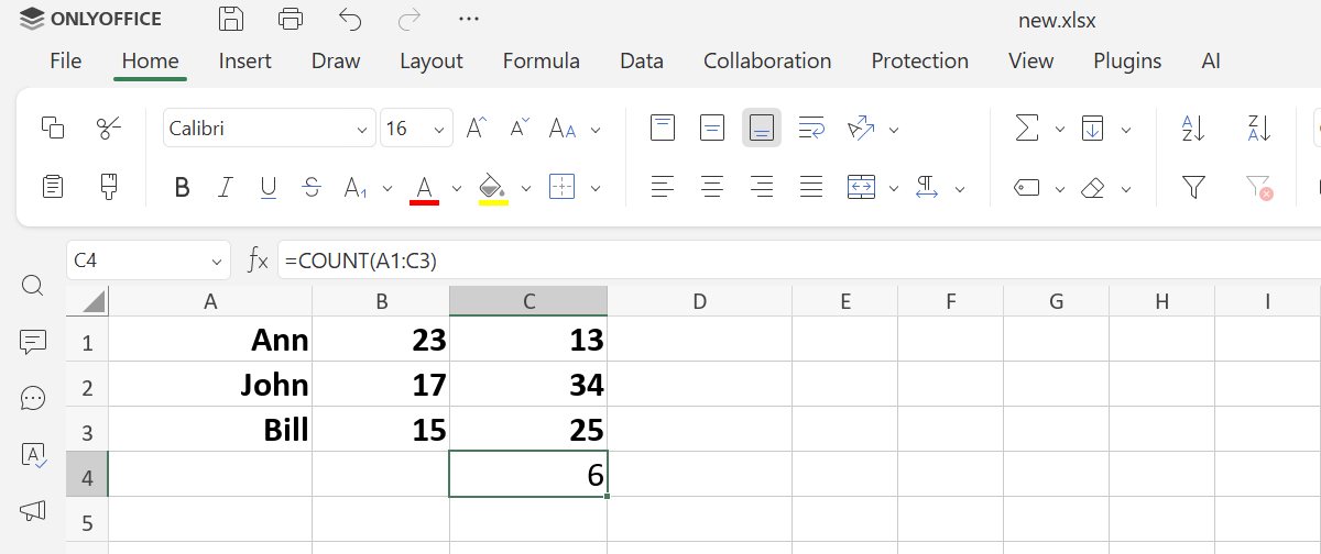
10. COUNT / COUNTA – Counting cells

COUNT counts numeric values; COUNTA counts all non-empty cells.

Syntax:

=COUNT(value1, value2, ...)

=COUNTA(value1, value2, ...)

Practical use: Survey analysis, tracking entries, validating data completeness.

Advanced tip: Don’t confuse COUNT with COUNTA; COUNT ignores text, COUNTA includes it.

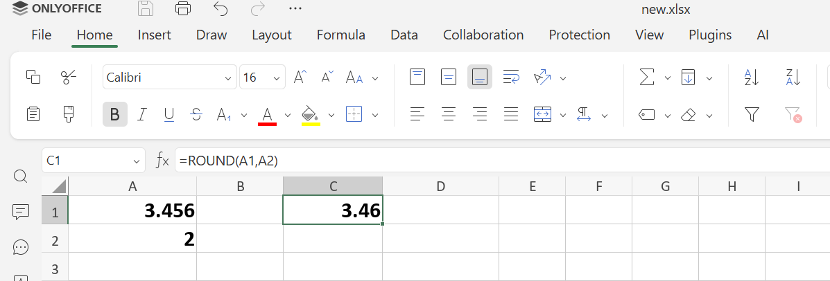
11. ROUND – Rounding numbers

ROUND rounds numbers to a specific number of decimal places.

Syntax:

=ROUND(number, num_digits)

Practical use: Financial reports, measurement simplification, standardized output.

Advanced tip: Use ROUNDUP or ROUNDDOWN to control rounding direction.

For further information about the formula, read our blog about it.

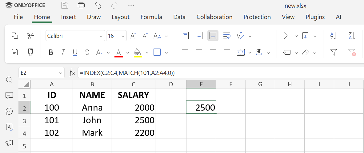
12. INDEX & MATCH – Flexible Lookup

Combines two functions to locate values anywhere in a table, offering more flexibility than VLOOKUP for complex data extraction.

Syntax:

=INDEX(return_range, MATCH(lookup_value, lookup_range, 0))

Practical use: Cross-referencing, multi-table dashboards, dynamic data extraction.

Advanced tip: Replace VLOOKUP with this formula when tables are rearranged or when the lookup value is not in the first column.

Get ONLYOFFICE Spreadsheet Editor

Put these formulas into practice with ONLYOFFICE Spreadsheet Editor and take full control of your data. Create structured workbooks, organize sheets efficiently, apply advanced functions, and work with complex calculations without compatibility issues. Manage financial reports, track projects, analyze performance metrics, and build accurate, professional spreadsheets in a reliable and intuitive environment.

If you don’t have an ONLYOFFICE account yet, sign up for free and start working with real Excel files right away. Use the editor directly in your browser for instant access from any device, or download the desktop app to manage your spreadsheets locally with full functionality.

START ONLINE   GET DESKTOP APP